RStudio as a Research and Writing Platform

Reproducible Research

In an 18-minute video, J.J. Allaire, Founder and CEO of RStudio, states:

Those who receive the results of modern data analysis have limited opportunity to verify the results by direct observation. Users of the analysis have no option but to trust the analysis, and by extension the software that produced it. This places an obligation on all creators of software to program in such a way that the computations can be understood and trusted.

This leads to the concept of reproducible research, “the idea that data analyses, and more generally, scientific claims, are published with their data and software code so that others may verify the findings and build upon them. The need for reproducibility is increasing dramatically as data analyses become more complex, involving larger datasets and more sophisticated computations. Reproducibility allows for people to focus on the actual content of a data analysis, rather than on superficial details reported in a written summary. In addition, reproducibility makes an analysis more useful to others because the data and code that actually conducted the analysis are available.”

The author of What is reproducible research? lists the following criteria:

A study can be truly reproducible when it satisfies at least the following three criteria.

– All methods are fully reported.

– All data and files used for the analysis are (publicly) available.

– The process of analyzing raw data is well reported and preserved.

An excellent reference is Reproducible Research with R and RStudio, Second Edition by Christopher Gandrud. The author has freely provided this book in reproducible form. Pre-compiled PDF versions can also be found in various internet locations, such as here.

This post will demonstrate the use of RStudio as a platform for the production of transparent, reproducible research. RStudio facilitates a form of the plain-text workflow in which you can write, cite the literature and produce formatted bibliographies, perform statistical analyses, create graphics, and execute code in R and several other programming languages, all from one, plain-text document. Because the document contains only plain text, it is futureproof, easily archived and shared, can be edited on any type of computing device, and is fully compatible with version control systems.

Software Installation

To use RStudio, you first have to install R. DO NOT install RStudio first. R has to be installed first, followed by RStudio.

To install R, go to the R Web site. Under “Getting Started:”, click download R. Choose a CRAN (Comprehensive R Archive Network) mirror site that is closest to you. This should bring you to a web page that looks something like this:

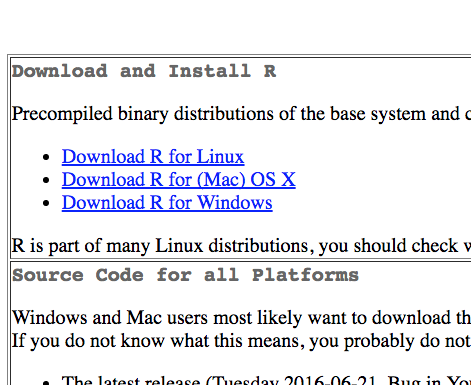
Under “Download and Install R,” download and run the installer (“Precompiled binary distribution”) for your particular computer platform. Follow the installation instructions and you should be off and running. Extensive gory details can be found at R Installation and Administration.

After installing R, there should be an R icon somewhere on your computer system, or perhaps an entry in an Applications folder or start menu. When you run R, you will be brought to the R console, which looks like this on an iMac:

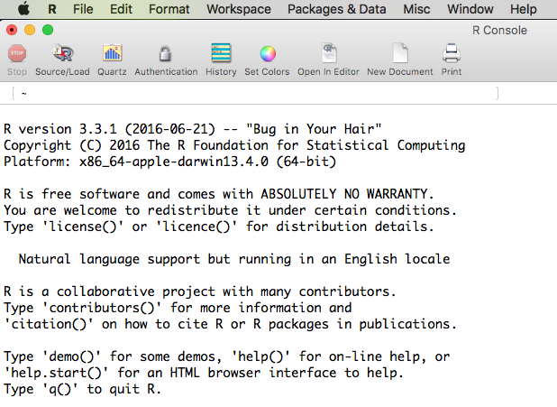
After briefly studying the R console, terminate R and forget about it, because we will be using R from inside of RStudio. We will not dwell on the details of using R; for that, please see An Introduction to R. We will focus instead on RStudio, which is what you need to install next. You must have R installed before you can use RStudio, but once RStudio is installed you do not need to have R running, as RStudio contains its own instance of R.

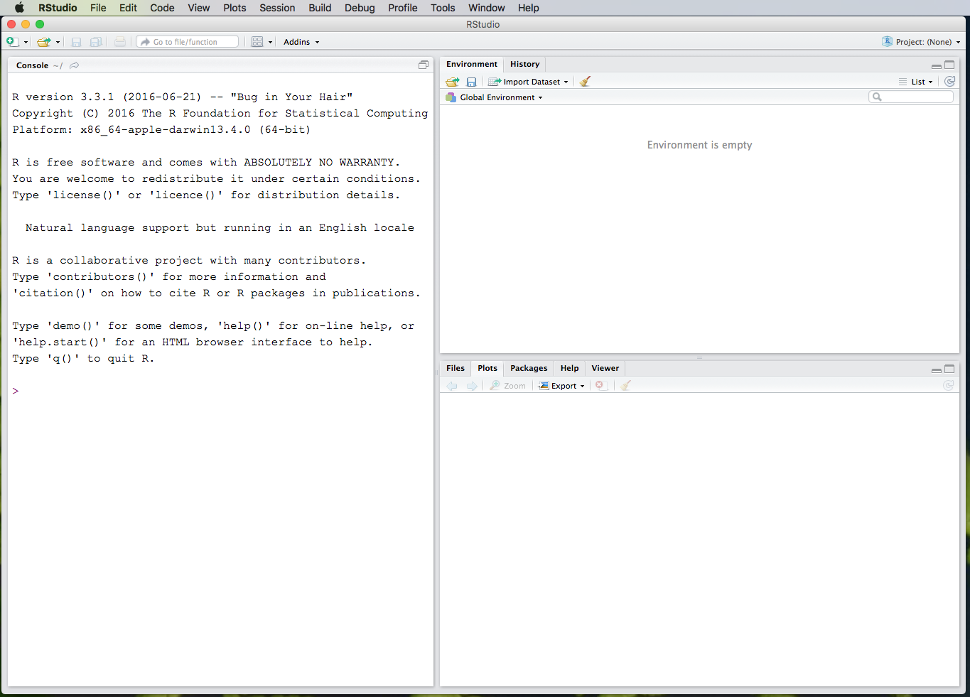
To install RStudio, go to the RStudio Desktop download site, and download and run the installer for your particular computer platform. After installation, run RStudio, and you should see something like this:

(Click image to enlarge.)

The above screenshot is from an iMac, but Windows and Linux users should find it comparable to RStudio running on their systems.

For PDF output in RStudio, you also need to install a version of the TeX typesetting system. Specifically, you need to install either MiKTeX on Windows, MacTeX 2013+ on OS X/macOS (best to download with Safari, and use the full version, not the smaller BasicTeX), or TeX Live 2013+ on Linux).

Rendering Documents in RStudio

We will first examine RStudio as a platform for writing plain text R Markdown documents, inserting bibliographic citations, producing formatted bibliographies, and rendering the Markdown document into publication-quality output.

Markdown is a lightweight markup language with a simple syntax designed to streamline the process of formatting and rendering plain-text documents. (See The Plain Text Workflow for a discussion of why you should be doing all of your writing in plain text instead of in a word processor.) While they can be rendered into many different publication-ready formats, including PDF, HTML, and Microsoft Word, Markdown files can stand on their own as human-readable text documents without being rendered. This is a big advantage for archiving and sharing, because no special software is needed to read Markdown and R Markdown files. Any plain-text editor¹ will do, and every computer already comes with one installed (TextEdit for Mac, Notepad for Windows, Emacs for Linux/Unix, etc.). RStudio has developed R Markdown, which preserves the syntax of the original Markdown but also allows the inclusion of blocks (“chunks”) of R code and code from several other programming, database, and scripting languages. R Markdown also has enhancements for tables, footnotes, citations, and other features of scholarly documents. As with the original Markdown, R Markdown is plain-text and human-readable, meaning that “anyone who has never even heard of R Markdown can understand what is happening to some extent.”²

Two handy PDF references for R Markdown are the R Markdown Cheat Sheet and the R Markdown Reference Guide. These two documents cover all that you will ever need to know about R Markdown syntax, options, and output formats. Here we will focus on the basic features that you will need to get started with RStudio and R Markdown.

As you work in RStudio, it’s possible that you will get messages about one or more R packages (for example, rmarkdown) not being installed. If this happens, just go to the Packages tab and install them. Click the Install button, search for the package name, be sure Install dependencies is checked, and install the missing packages. RStudio may also present a message saying that it wants to install required or updated packages. Say Yes.

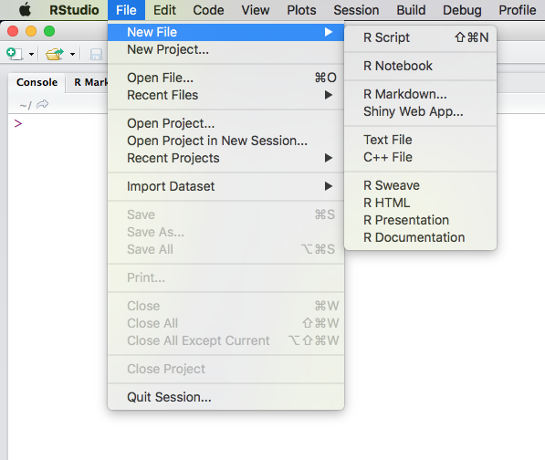
RStudio provides templates for both R Markdown and R Notebooks. In RStudio, click the File menu, then select New File:

(Click image to enlarge.)

Choose R Markdown, give the document a title, and a text editor window will then open containing the R Markdown template:

(Click image to enlarge.)

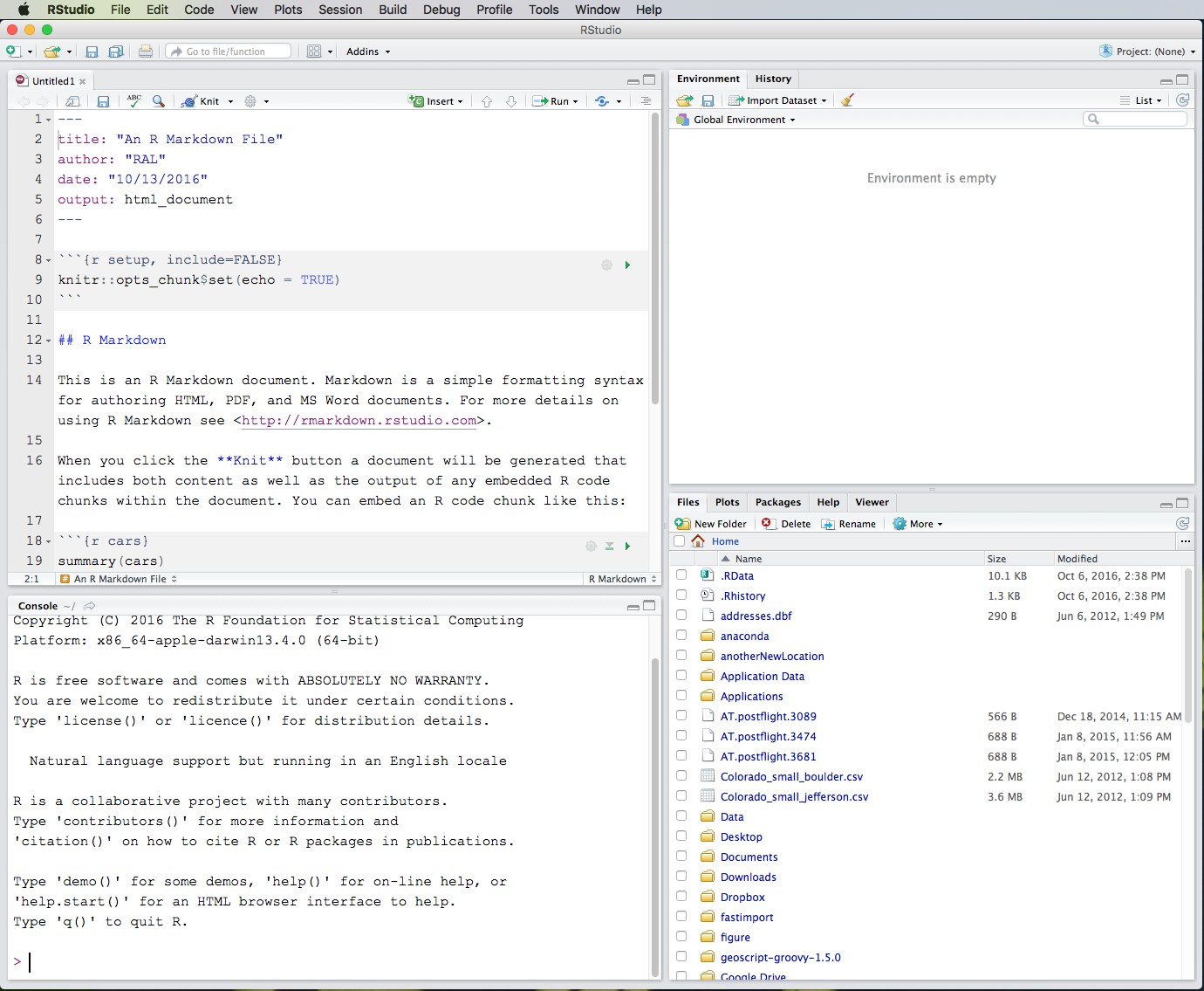
You should now have 4 panes open in RStudio. The content of the panes can be customized under Pane Layout in RStudio Preferences. What you see in the above screenshot is the default layout. The upper-left pane is a text editor containing the R Markdown document we just created. This editor can also be used to create R scripts and various other plain-text source files. Below the editor is a pane containing the R Console. This is exactly the same console that you would get if you ran R by itself, independently from RStudio. (The Console pane contains an instance of R running inside of RStudio. You can have multiple instances of RStudio running at once, each running its own separate instance of R.) You can enter R commands directly into the Console, and text output from R commands will also appear here. In the upper right pane are tabs for the Environment (containing variables and other data structures created during the session) and History (a list of all R commands entered during the session). In the lower-right pane are tabs for Files (your computer’s filesystem), Plots (graphics created by R), Packages (a tool for installing and updating R packages), Help (the R help system), and the Viewer (containing output from rendering R Markdown files and R Notebooks).

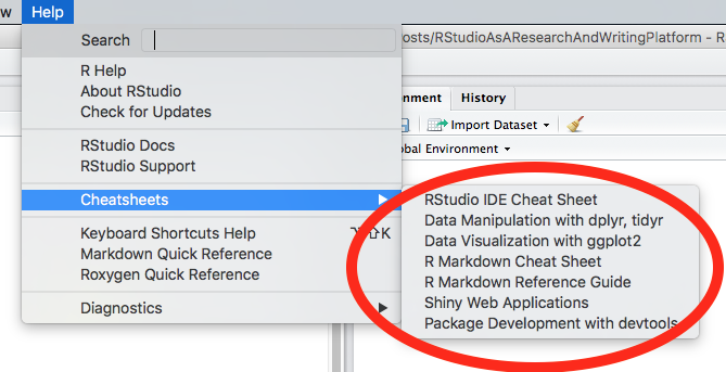
Of course, there is a very nice RStudio Cheat Sheet. The RStudio Help menu has links to additional very nice cheat sheets:

(Click image to enlarge.)

You can also access a Markdown Quick Reference from the RStudio Help menu. This will open up in the RStudio Help tab. You can copy-paste Markdown syntax from the Quick Reference into your R Markdown document. (Sadly, RStudio does not have Markdown syntax built into its editor, at least at the time of this writing.)

The first part of the as-yet-unnamed R Markdown file looks like this:

---
title: "An R Markdown File"
author: "RAL"
date: "10/14/2016"
output: html_document
---

This is called the YAML header. YAML (YAML Ain’t Markup Language) is a human friendly data serialization standard for all programming languages. In R Markdown, the YAML header (which is optional) is placed at the top of the document between lines that start with three dashes (---) and contains metadata for the document (e.g., title, author, date) and other options that control how the document is rendered.

Besides the YAML header, R Markdown documents contain either text or code chunks. Text is formatted using R Markdown syntax. R code chunks are made with three backticks immediately followed on the same line by an r in braces. End the chunk with three more backticks, on a separate line:

```{r comment=""}
paste("Hello", "World!")
```

[1] "Hello World!"

The backtick symbol is located to the left of the numeral 1 on your keyboard. It is NOT a single apostrophe (').

Additional R options can be placed inside of the braces, for example:

```{r, echo=FALSE, comment=""}
    summary(cars)
```

     speed           dist       
 Min.   : 4.0   Min.   :  2.00  
 1st Qu.:12.0   1st Qu.: 26.00  
 Median :15.0   Median : 36.00  
 Mean   :15.4   Mean   : 42.98  
 3rd Qu.:19.0   3rd Qu.: 56.00  
 Max.   :25.0   Max.   :120.00  

The R option echo=FALSE will display the output of a code chunk but not the underlying R code. The comment="" option turns off the default ## that usually precedes each line of output.

All of the R code for a chunk must be inside of the space defined by the two lines of backticks.

At the top of the editor window is a toolbar:

(Click image to enlarge.)

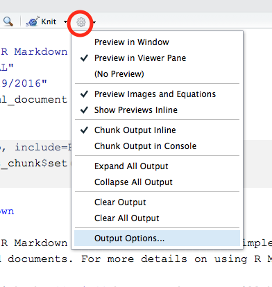
Drop down the menu next to the Knit icon, and you will see options for rendering the R Markdown document into publication-quality output:

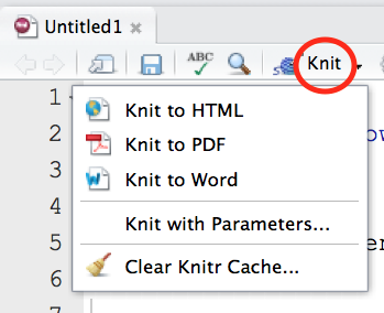
This function is called Knit because it invokes an R package called knitr that “knits” the Markdown-formatted text, relevant YAML content, and R code chunks together into a rendered document.

Try knitting the document into HTML, PDF, and Word formats. You will first need to give the R Markdown file a name, if you haven’t already done so. The default R Markdown file name extension is Rmd. The HTML rendering will appear in the RStudio Viewer pane. If it appears in a separate window, drop down the gear icon next to the knit button and select Preview in Viewer Pane. PDF output will open in a separate PDF viewer window. When you render the document to Microsoft Word format, it will open up in Microsoft Word. HTML, PDF, and Word files having the same name as your R Markdown document will be saved in your working directory.

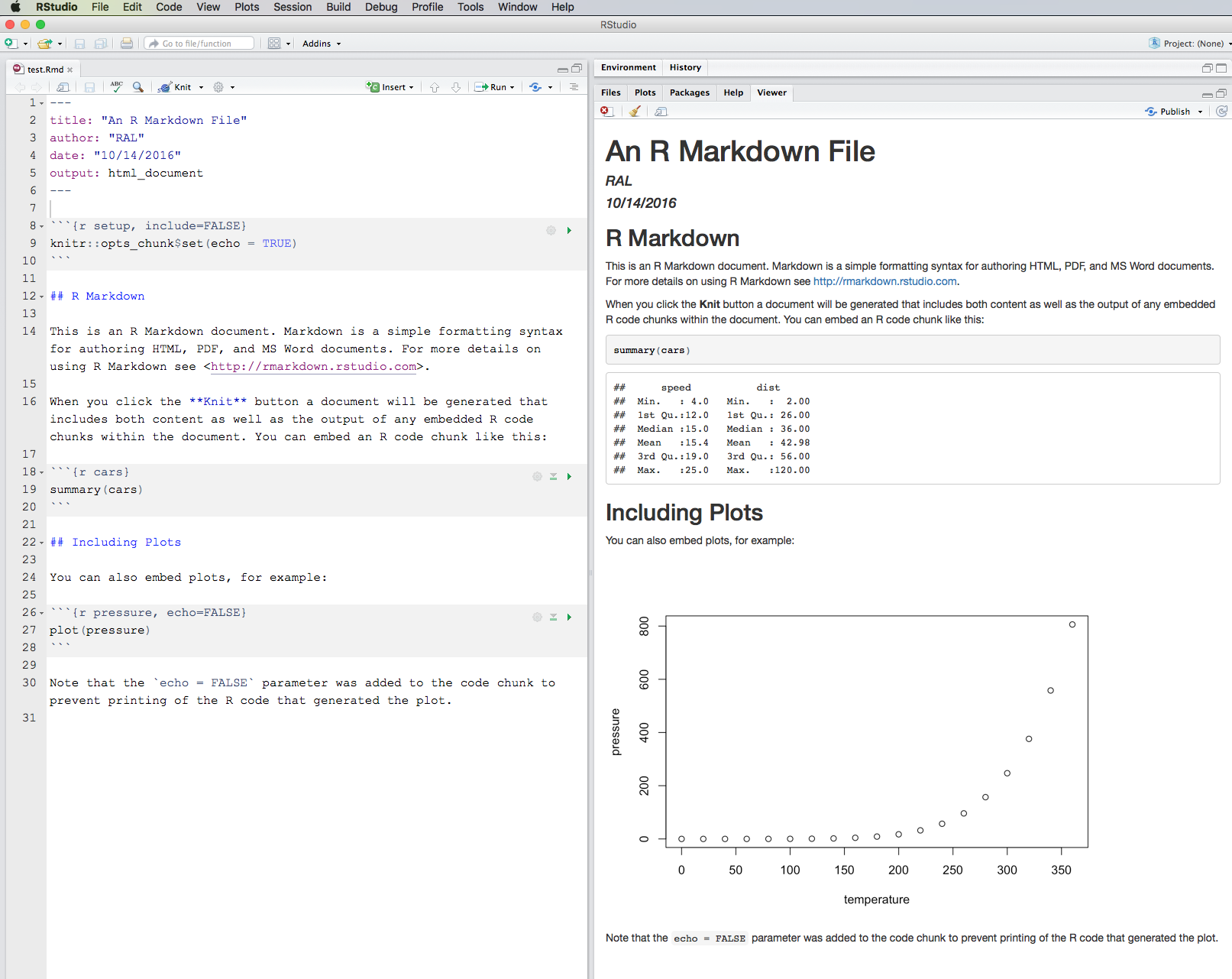
Let’s look at an HTML rendering:

(Click image to enlarge.)

In the above screenshot I have maximized the Editor and Viewer panes so we can see them side-by-side. The title, author, and date contained in the YAML header appear in the rendered document, but the YAML statement output: html_document does not because it is a formatting command, not printable text. Regular text appears in the HTML as formatted by R Markdown syntax. Text and graphical output produced by R code chunks appears in the rendered document at the point where the code chunks were placed in the original R Markdown document. Display of the code itself can be turned off in the rendered document by use of the echo=FALSE parameter in the code chunk:

```{r pressure, echo=FALSE}
    plot(pressure)
```

If you knit the R Markdown document to HTML, PDF, and Word formats, you will notice that the YAML header in the R Markdown document has been modified:

---
title: "An R Markdown File"
author: "RAL"
date: "10/14/2016"
output:
  word_document: default
  pdf_document: default
  html_document: default
---

RStudio inserts additional formatting parameters into the YAML header to control how the document is rendered. You can do this manually as well, simply by editing the YAML header directly, in the editor. For example, to control the size of R graphics in Microsoft Word, add this to the YAML header:

output:
  word_document:
    fig_width: 3
    fig_height: 3

This will cause figures in the resulting Word file to be sized at 3 by 3 inches. You can also set YAML options interactively, by clicking the gear icon to the right of the Knit button, and choosing Output Options:

This will give you a dialog box from which you can choose the various output formats and set things like figure size, inclusion of figure captions, etc.:

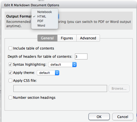
When you make selections from the Output Options dialog, RStudio will make the appropriate changes to the YAML header in the R Markdown document. You can also edit those parameters directly in the YAML header, as mentioned earlier.

See RStudio Formats for more formats and YAML options for rendering R Markdown documents.

Writing and Citing in RStudio

For this example I am using a new R Markdown file, created using the RStudio template as demonstrated above, but with everything deleted except the YAML header. I have titled the document “Our Friend the Catbird”³ and have also deleted the YAML author and date fields to keep things simple. I have named the file citations.Rmd, but any file name will do as long as you use the .Rmd filename extension.

Thus the YAML header currently looks like this:

---
title: "Our Friend the Catbird"
output: html_document
---

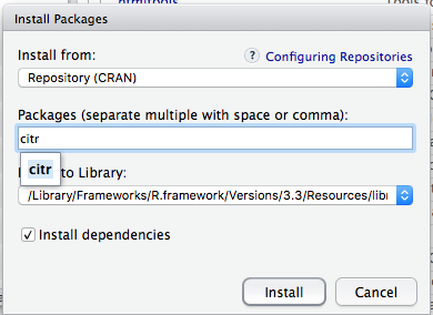
In RStudio, inserting literature citations and creating formatted bibliographies in R Markdown documents is facilitated by an R package called citr. To install it, go to the Packages tab in RStudio, click the Install button, enter citr into the search bar, be sure that Install dependencies is checked, and then click Install:

If you then click the Addins button on the main RStudio toolbar, you should see an entry for Insert citations:

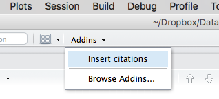
If you don’t see Insert citations, be sure that citr is checked in the list of installed packages in the Packages tab. You might have to restart RStudio after checking citr in the package list.

Before we can use citr, we need a BibTeX bibliography file.

Here’s one: references.bib.

To follow along with this example, click the above link and download references.bib to your RStudio working directory, or some other location where you can find it.

BibTeX files are plain text and can be created by the major reference manager applications, such as RefWorks, EndNote, Mendeley, and Zotero. Many other reference manager applications, e.g. JabRef, use BibTeX as their native format; see Comparison of reference management software. The BibTeX format is widely used and has been around for a long time.⁴

A BibTeX reference entry looks like this:

@article{marsh_adaptations_1984,
  title = {Adaptations of the {{Gray Catbird}} to Long Distance Migration: 
  Flight Muscle Hypertrophy Associated with Elevated Body Mass},
  volume = {57},
  timestamp = {2016-03-12T15:29:37Z},
  number = {1},
  journaltitle = {Physiological Zoology},
  author = {Marsh, R. L.},
  date = {1984},
  pages = {105--117}
}

All reference manager applications break bibliographic citations into a series of fields that can be reassembled into any citation style desired, such as that of the journal Ecology:

Marsh, R. L. 1984. Adaptations of the Gray Catbird to long distance migration: 
Flight muscle hypertrophy associated with elevated body mass. Physiological Zoology 57:105–117.

The references.bib file used in this example was created by exporting references from Zotero using the BibTeX export translator.

The YAML header can contain the name of a BibTeX file to use for literature citations. Thus we add bibliography: references.bib to our YAML header so that it now looks something like this:

---
title: "Our Friend the Catbird"
output: html_document
bibliography: references.bib
---

This assumes that references.bib is in the same folder as the R Markdown file. But you could also store references.bib in some other location, as long as you provide the complete path to the file, for example:

bibliography: /User/rlent/Desktop/references.bib

You can also provide multiple BibTeX files in the YAML header by listing them like this:

bibliography: [statistics.bib, graphics.bib]

And so, with bibliography: references.bib added to the YAML header of citations.Rmd, and with the references.bib file residing in the same folder as citations.Rmd, click Addins, then select Insert citations. A dialog box should appear:

(Click image to enlarge.)

Note that we get an acknowledgement that references.bib was found in the YAML header. An error message will appear in the search bar if there was a problem finding the bibliography file. If you click in the search bar, where it says Search terms, you should see a scrollable list of the references contained in references.bib:

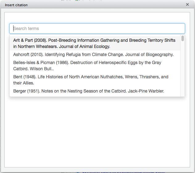
(Click image to enlarge.)

You can select one or more references from the list, by clicking on them, and the selected references will be added to a separate box above the scrollable list:

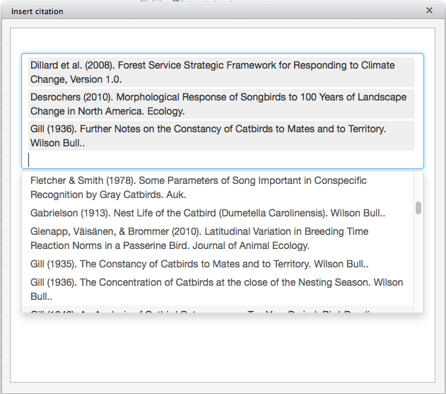
(Click image to enlarge.)

When you are finished selecting references to cite, click in a blank area of the dialog box, and citr will build a citation marker to insert into your text:

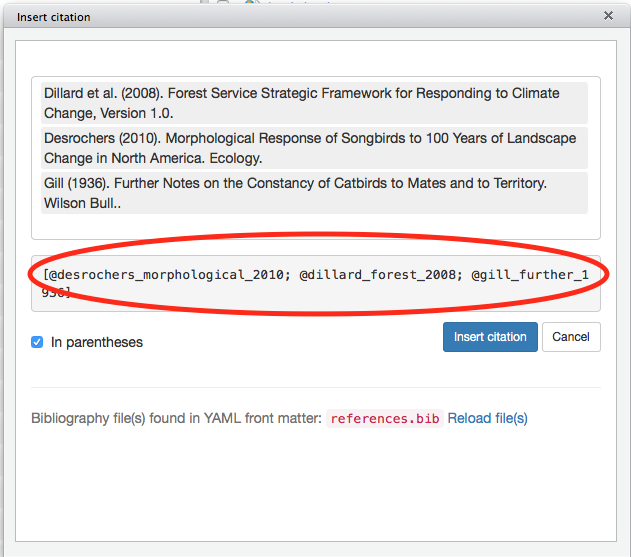
(Click image to enlarge.)

The citation marker consists of one or more BibTeX citation keys, each beginning with the @ symbol, each separated by semicolons, with everything enclosed in square brackets. The citr tool takes care of this in-text formatting automatically; all you have to do is select the references you want to cite.

Each reference in a BibTeX file contains a citation key at the beginning of the entry:

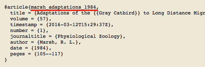
(Click image to enlarge.)

The citation key uniquely identifies each reference in the BibTeX file and is used as a place marker for in-text citations in the R Markdown file.

By default, RStudio will use a Chicago author-date format for citations and references. To use another style, you need to specify a CSL (Citation Style Language) style file in a csl metadata field in your YAML header. CSL styles are plain-text and are written in XML. You can select and download over 8300 CSL bibliographic styles from the Zotero Style Repository.

Let’s first try citing using the default style. This means that our YAML header looks like this:

---
title: "Our Friend the Catbird"
output: html_document
bibliography: references.bib
---

Here the YAML header only specifies the BibTeX file, and does not specify a particular CSL style file. Therefore the default Chicago author-date style will be used.

We type some text, and leave our cursor at the point in the text where we want to insert a citation:

(Click image to enlarge.)

We then click Addins|Insert citations, and search for a reference to cite:

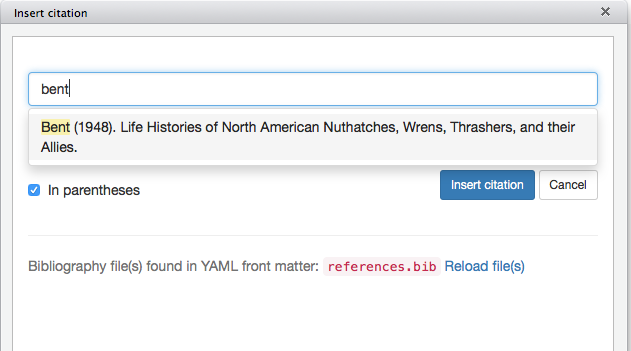
(Click image to enlarge.)

Be sure In parentheses is checked (this puts in the square brackets), click Insert citation, and the citation marker will be inserted into your text at the current cursor position:

The catbird is one of our most beloved songbirds [@bent_life_1948].

Now, if we knit the R Markdown document to HTML, it looks like this:

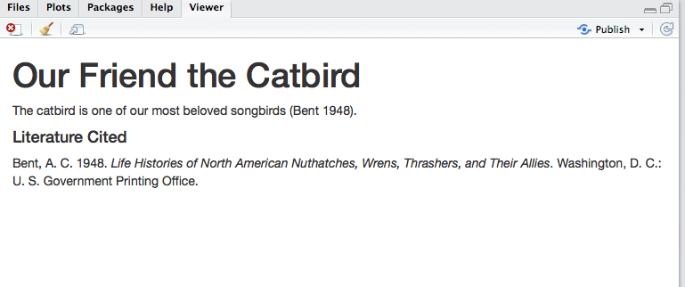
(Click image to enlarge.)

RStudio, via the citr package and another application called pandoc (automatically installed with RStudio; see also Pandoc Markdown), has changed the citation marker to the appropriate in-text citation style (in this case, the default Chicago author-date style) and has created a formatted bibliography, also in the Chicago style. The bibliography is always placed at the end of the document; I had already inserted a Markdown heading (#### Literature Cited) to create a Literature Cited section.

If we want a specific bibliographic style other than the default Chicago style, we need to add a csl metadata entry to our YAML header:

---
title: "Our Friend the Catbird"
output: html_document
bibliography: references.bib
csl: nature.csl
---

The csl: nature.csl YAML entry points to a CSL style file called nature.csl that was downloaded from the Zotero Style Repository. This is the style used in the journal Nature.

(Here is nature.csl if you want to download it for this example.)

Now, when we knit to HTML, we get:

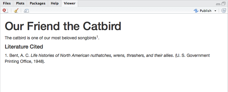
(Click image to enlarge.)

The rendered HTML has been reformatted to follow the bibliographic style specified by nature.csl. In-text citations are now numbered superscripts, and the bibliography is also numbered and organized in citation order instead of alphabetically by author’s last name. (This would be more obvious if we had more than one citation.)

See Bibliographies and Citations for more information on citing and creating bibliographies in RStudio. For example, using an author-date style like Chicago, if you put a minus sign before the opening @ of a citation key in the text, like this:

[-@bent_life_1948]

you can suppress the author’s name in the citation. Now we can write a sentence that reads:

Arthur Bent (1948) said that the catbird is one of our most beloved songbirds.    

An R Markdown Template for Academic Manuscripts provides more useful tips on YAML and R Markdown documents.

R Notebooks

An R Notebook is an R Markdown document with a special execution mode for interactive data analysis. Any R Markdown document can be used as a notebook, and R Notebooks can be rendered into the same publication-quality document formats as regular R Markdown files. By default, RStudio enables notebook mode on all R Markdown documents, so you can interact with any R Markdown document as though it were a notebook.⁵ R Notebooks, however, offer additional features that are not available in regular R Markdown documents.

In RStudio, create a new R Notebook by clicking the File menu, then New File, and then select R Notebook. For this example we will save the notebook and give it a file name of MyNotebook.Rmd. Your editor pane should now look something like this:

(Click image to enlarge.)

This is the R Studio template for an R Notebook. Kind of looks like regular R Markdown, doesn’t it? That’s because an R Notebook is an R Markdown document with code chunks that can be executed independently and interactively. Text and graphical output will appear immediately beneath the code chunk that produced it, in the editor window.

You can execute your notebook code chunks interactively by using the controls that appear in each chunk:

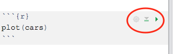
The rightmost arrow will run the current chunk. To the left of the run arrow is a down-pointing arrow that will run all of the chunks above the current chunk. The gear icon allows you to modify options for how each code chunk behaves. These same controls are also available in regular R Markdown documents.

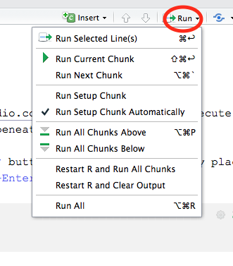
More options for running code chunks can be found in the Run menu on the editor toolbar:

A feature unique to R Notebooks is notebook Preview:

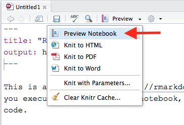
While an R notebook preview looks similar to a rendered R Markdown document, the notebook preview does not automatically execute and knit all of your code chunks, which is what happens when you render an R Markdown document. A notebook preview simply shows you a rendered copy of the Markdown text in your R Notebook along with the most recent chunk output. This allows you to efficiently develop R code in an R Notebook by iterating back and forth between coding and output until the code chunk is completed, without having to render the entire document each time you want to look at the output of a single code chunk.

Try previewing the R Notebook template before running the embedded code chunk. You’ll see just the text of the notebook in the Viewer pane. Then run the code chunk by clicking the Run arrow. A plot of the cars dataset (which comes with R) will appear immediately below the code chunk, not in the View pane, but right in the editor window. In the upper right corner of the plot window are tools for clearing the output, expanding or collapsing it (without clearing it), and for opening the graphic in an external window. If you leave the plot displayed, and then preview the notebook, you will now see the graphic included with the rendered text.

The YAML header in our R Notebook looks like this:

---
title: "R Notebook"
output: html_notebook
---

The output: html_notebook statement in the YAML header is what turns a regular R Markdown document into an R Notebook. So if you start out with an R Markdown document and then decide that you want to “upgrade” it to a notebook, just add output: html_notebook to the YAML header. This will turn your R Markdown document into an R Notebook and will also turn the Knit button into a Preview button. You will still have the option to knit the notebook completely into publication-quality output with all R text and graphical output. Just pull down the Preview button and you will see the knit options for HTML, PDF, and Word output.

Now that you have previewed MyNotebook.Rmd with the chunk output displayed, note that there is a file named MyNotebook.nb.html in your working directory. As discussed here, when a notebook .Rmd file is saved, the output: html_notebook statement in the YAML header causes an .nb.html having the same name as the notebook to be saved as well (the nb stands for notebook). This file is a self-contained HTML document having both a rendered copy of the notebook with all current chunk outputs (suitable for display on a website) plus a copy of the notebook .Rmd source file itself.

Open your RStudio Files pane, and click on MyNotebook.nb.html in the list of files. Choose to view the file in a web browser. It should look something like this:

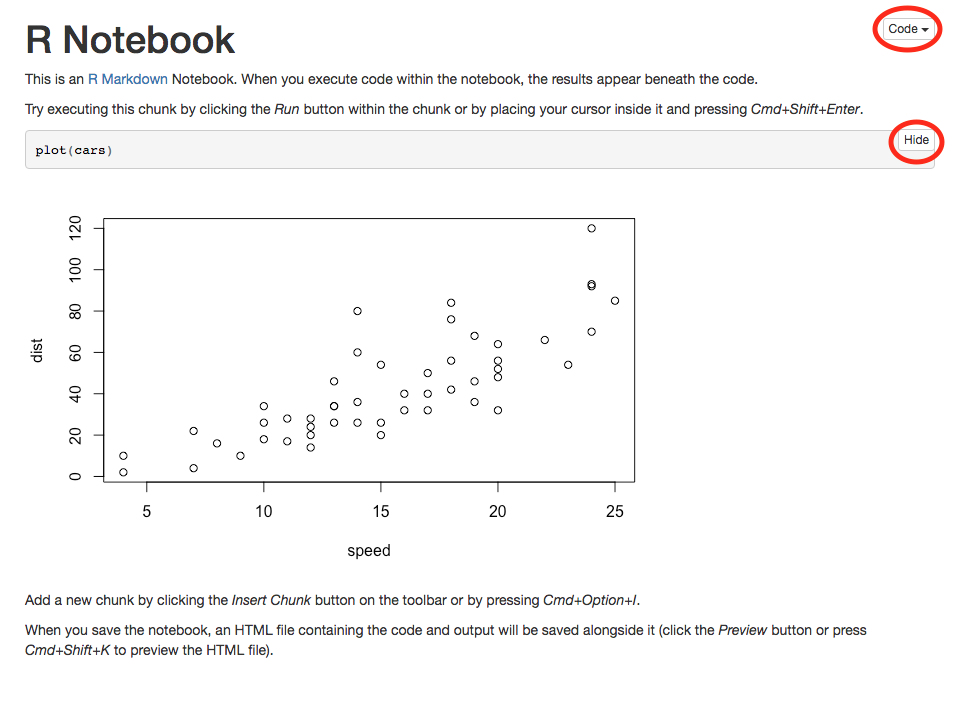
(Click image to enlarge.)

In this web page, there is a button labeled Hide that you can use to show and hide the code that produced the plot. There is also a button labeled Code that lets you show and hide all of the code and also lets you download the original notebook .Rmd file.

The nb.html files are an excellent way to archive and share R notebooks. Anyone with access to an nb.html file has a complete package of the rendered text of the notebook, all of the tabular and graphical output from the code chunks, and a copy of the original R Notebook .Rmd file. Because the nb.html file can be viewed in any web browser, a person does not have to have R or RStudio in order to view the notebook, the code, or the output. However, if one of your collaborators does have RStudio, they can open the nb.html file directly using the File|Open File... dialog of RStudio to resume work on the notebook with all output intact. This will extract the .Rmd file into a new RStudio editor tab, extract the chunk outputs from the .nb.html file, and place them appropriately in the editor.

Only R Notebooks (which have at least one of the output formats in the YAML header listed as html_notebook) can produce a companion .nb.html file. Regular, non-notebook R Markdown files can have inline chunk output (the chunk output appears immediately below the chunk, in the editor) but they do not produce an .nb.html file.

Reproducible Research Revisited

If we were creating a journal article back in the olden days (i.e., prior to 2011, the first public beta release of RStudio), we would start writing our manuscript in a word processor, say Microsoft Word. If it was a science manuscript, the text would contain Introduction, Methods, Results, Discussion, and Literature Cited or References sections. The data, say from a laboratory experiment or from field observations, might reside in an Excel spreadsheet, a database application, or preferably in one or more plain text files. To produce data summaries, statistical analyses, and graphics, we would have to bring the data into a statistics package like SPSS, SAS, or one of many others. Reduction and manipulation of the original data might continue in the statistical software. Tabular statistical output such as regression and ANOVA tables would need to be copy-pasted back into Word, where they might then be wrangled into a pretty table. Graphical output from statistical software or maybe a separate graphics package would need to be saved to a graphics file, then imported back into Word. If we needed a map of study sites, we might have to use a geographic information system to produce a map, requiring even more data files, and then export the map to an external graphics file so that it could be brought into Word. Bibliographic references might be stored in reference management software like Zotero or RefWorks, and via a Word plugin, we could produce our literature citations and formatted bibliographies. At some point, a final manuscript would be produced.

And then the revisions would begin.

The cut-and-paste approach to producing a scholarly manuscript is tedious, slow, and error-prone, to say the least. Moving data back and forth between applications makes it difficult to retrace the steps taken to produce a given result, even if careful notes are taken every step of the way. If a project involves multiple researchers, each working on different parts of the analysis, and each keeping their own set of notes, this process becomes even more complicated.

Production of an analysis, publication-quality graphics, and a final manuscript can be greatly streamlined by keeping everything in one R Notebook. With R code chunks embedded in R Markdown text, you can fully document how you arrived at your results, while simultaneously producing the statistical output, graphics, and references for your paper. R Notebooks can be easily archived and shared among collaborators, using cloud storage technologies such as Dropbox and Google Drive, or version control systems such as git, and can be rendered into publication-quality documents in a variety of formats. And because everything is plain text, the R Markdown manuscript can be edited on any computing device that has a text editor, including smartphones and other mobile gadgetry.

We illustrate this workflow with a small example, involving the analysis of the raw data file sites.csv. This is a comma-separated values file containing ecological data from 11 grassland sites in Massachusetts, New Hampshire, and Vermont. The companion metadata file sites.metadata.txt describes the variables (columns) of sites.csv. The data for each site consist of measures of site vegetation structure, morphological measures on individuals of the butterfly species Coenonympha tullia (the Common Ringlet) inhabiting each site, and the geographic location of each site in both UTM and decimal degree coordinates. The aim of the study was to examine relationships between habitat structure and morphological variation in the butterfly populations at each site.

You can view the complete example in sites.nb.html, which is an HTML notebook created in RStudio from the corresponding R Notebook file sites.Rmd. The HTML notebook contains the rendered text of a scientific paper originally written in R Markdown with embedded R code that creates all of the statistical analyses, tables, and graphics. The same sites.Rmd file was used to produce PDF and Microsoft Word versions of the paper. The manuscript in sites.Rmd was written to be self-contained and self-documenting, essentially a “paper-within-a-paper.” It includes comments that document both the main text and the embedded R code. Also in sites.nb.html is a link from which you can download a copy of the complete R Markdown source file sites.Rmd. You can also download sites.zip, a zip archive file that contains all of the document files, data, metadata, R code, and other associated files (such as external images and bibliographic data) needed to replicate our example analysis and document production.

Recalling the 3 criteria for reproducible research, the files comprising our example satisfy the requirement that All data and files used for the analysis are publicly available. The data file and its companion metadata file would be placed in a publicly accessible digital repository so that other workers desiring to replicate the analysis could get the data and know what they were working with. At a minimum, the metadata file needs to describe what the variables are and their units of measurement. The requirement that All methods are fully reported should be satisfied by the Methods section of the article. Because the article is written in R Markdown and contains embedded R code showing exactly how the data were analyzed, we also have satisfied the third requirement of reproducible research, that The process of analyzing raw data is well reported and preserved. The R Markdown manuscript with its embedded R code and accompanying data and metadata files, all residing in sites.zip, is a self-contained package of reproducible research.

Coda I: Python

We note briefly here that you can insert code chunks from other programming languages besides R into an R Markdown document. See knitr Language Engines for more details. There is an example of an R Notebook that includes both R and Python code here.

Coda II: Inspirational Quotes About Data

“Data! Data! Data!” he cried impatiently. “I can’t make bricks without clay.” – Sherlock Holmes, The Adventure of the Copper Beeches

“War is 90% information.” – Napoleon Bonaparte

“Everybody gets so much information all day long that they lose their common sense.” – Gertrude Stein

“Statistics are no substitute for judgment.” – Henry Clay

“Information is not knowledge.” – Albert Einstein

“Facts are stubborn, but statistics are more pliable.” – Mark Twain